What we borrowed in ML from info theory

Information Theory

Random Variables

A random variable is a mapping from the object space (denoted as the set \( \Omega \)) to \( \mathbb{R} \) (the set of real numbers), and it depends on a random event. An example in machine learning is the label produced by a classification system. Assuming a binary classification problem, the label can be either positive (mapped to \( 1 \)) or negative (mapped to \( 0 \)), each occurring with a certain probability.

Information Content

Now think about how knowing the state of a certain random variable conveys information to you. Are you really excited to learn that you will wake up tomorrow? Probably not — this is a highly probable event, and you're almost certain it will happen. Because of that certainty, learning this fact doesn't feel surprising or informative.

On the other hand, if I told you that tomorrow you will not wake up — that would likely trigger a strong reaction. The event induced by the random variable (waking up or not) now lands on the unlikely outcome. Since it's unexpected, it feels surprising. Statistically speaking, this kind of event conveys a large amount of information.

We define the information content of an event with probability \( p_i \) as:

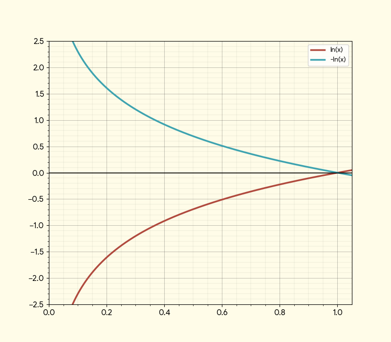
\[ I(p_i) = -\log(p_i) \]

Entropy

Now let's take a look at the entropy of a random variable. At its simplest, entropy is defined as the expected value of the information content of that variable. In other words, it tells us, on average, how much information the random variable provides across all possible outcomes.

If the entropy value is small, it means that a few events dominate with high probability. There's a sense of certainty — the variable doesn't surprise you often.

On the other hand, a higher entropy value suggests a flatter probability distribution. There are no sharp spikes, and many low-probability events could occur, which points to a higher level of uncertainty in the system.

Mathematically, the entropy \( H(X) \) of a discrete random variable \( X \) with probabilities \( p_i \) is defined as:

\[ H(X) = -\sum_i p_i \log(p_i) \]

Coding Scheme Interpretation

Before we move on, let me tell you about another interpretation of entropy. For this, I'll introduce the idea of a coding scheme — which, for now, you can think of as a way to represent the outcomes of a random variable in binary form.

Imagine you work at a company with three types of employees: full-timers, part-timers, and contractors. Your friend Claude, who sits in the other room, wants you to notify him every time an employee enters the office — but he wants you to send the information using binary strings. Claude only uses a pager, so he asked you to send the data using the least number of bits possible.

You're not as clever as Claude, so you ask for some tips. Given the three employee types, should you assign the same number of bits to each of them? Not really.

You know that full-timers are very common, so you assign them the shortest binary code. Part-timers are less common, so you assign a slightly longer code. Contractors are rare, so they get the longest code.

Shannon came up with a function that tells you the optimal number of bits needed to encode each outcome:

\[ \text{Bits}(p_i) = \log_2\left(\frac{1}{p_i}\right) = -\log_2(p_i) \]

So, the entropy of the random variable is the average number of bits needed to represent its outcomes under this optimal coding scheme:

\[ H(X) = -\sum_i p_i \log_2(p_i) \]

Cross-Entropy

Cross-entropy is a very similar concept in nature, but it assumes that we are using an imperfect tool to estimate the number of bits. To make this simple: imagine we are sampling outcomes from a random variable that follows some true distribution, where each sample has a true probability \( y \). However, we have a belief that the probability is \( y' \). Cross-entropy measures how bad that belief is.

Formally, it quantifies the error or cost of using the wrong coding scheme based on \( y' \) to represent a random variable that actually follows the distribution given by \( y \). In this sense, cross-entropy reflects how many bits you need when using a non-optimal coding schema. It is important to note that cross-entropy itself is not a comparison — it directly measures the number of bits required under the wrong schema, not how far it is from the optimal one.

The cross-entropy between the true distribution \( y \) and the estimated distribution \( y' \) is given by:

\[ H(y, y') = -\sum_i y_i \log(y'_i) \]

KL Divergence

Now that we defined some terminologies, KL divergence — or Kullback-Leibler Divergence — measures how many extra bits you need. It's the difference between the cross-entropy (the amount of bits needed using the incorrect coding schema) and the entropy (the amount of coding you'd want under the optimal schema):

\[ D_{KL}(y \,||\, y') = H(y, y') - H(y) \]

The full formula for KL divergence is:

\[ D_{KL}(y \,||\, y') = \sum_i y_i \log\left(\frac{y_i}{y'_i}\right) \]

Minimizing cross-entropy is equivalent to minimizing the KL term.

To not make math people unhappy, I need to note that KL is not a measurement or distance function, since it's not symmetric. And you might ask why it's not, while the fundamental operation is subtraction. The answer is that cross-entropy in itself is not symmetrical.

Mutual Information

This shows up more in classic machine learning, but I'll end by talking about mutual information — which measures the KL divergence between \( p(x, y) \) and \( p(x)p(y) \). If it's zero, you're basically saying both quantities are equal, which defines independence between the two random variables.

Let's write the conditional probability:

\[ p(y \mid x) = \frac{p(y \cap x)}{p(x)} \]

Now, if \( p(y \cap x) = p(y)p(x) \), then:

\[ p(y \mid x) = \frac{p(y)p(x)}{p(x)} = p(y) \]

So knowing about \( x \) doesn't convey anything about \( y \). For independent events, this is exactly what you expect — the probability doesn't change. But if the joint probability \( p(x \cap y) \) is different from \( p(x)p(y) \), that means knowing one tells you something about the other.

Hence, mutual information exists, and it's in the order of \( p(x \cap y) \), measuring how much the joint distribution deviates from independence.